An introduction to continuous conditional probability distributions

HTML-код
- Опубликовано: 7 сен 2024
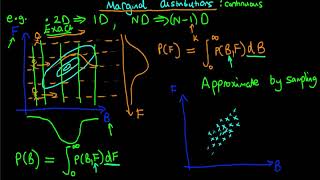
- An introduction to the concept of conditional probabilities via a simple two-dimensional continuous example.
This video is part of a lecture course which closely follows the material covered in the book, "A Student's Guide to Bayesian Statistics", published by Sage, which is available to order on Amazon here: www.amazon.co....
For more information on all things Bayesian, have a look at: ben-lambert.co.... The playlist for the lecture course is here: • A Student's Guide to B...


I'm so grateful that you continue making videos as you did. Thank you for your great effort. You have inspired a lot of learners like me!!
Thanks for these videos! They are great!
This is the point where things started to get confusing for me. I would welcome always clarifying when using expressions like P(A|B=b) whether this specific expression represents a 2D PDF, 1D PDF or a number. That way it would be clearer what type of object we divide by what type of object and what the resulting object's type is.
This expressions return 1D PDF; Basically 1D PDF/ Number
@@Theviswanath57 @ondrej havlicek It gets confusing because in the continuous case you deal with infinitely small changes and therefore the number that you divide the 1D PDF to normalize it is a very small number (tends to zero) so you can not really imagine how that will work using everyday intuition (and therefore you have to trust mathematicians that things work out just fine). Once you start dealing with infinity everyday intuition is no longer much helpful and confusion becomes the new normal I guess...
Confused how this differs from marginal probabilities. In the marginal case, I am imagining a horizontal plane through the contour plot where F is held constant (say F=f) and then integrating over B to obtain the marginal probability for F=f. How does this differ to a conditional probability, where I am determining say P(B|F=f)?
I was wondering the same thing.
After some pondering I realised that when you marginalise to get the marginal distribution of B you basically ignore F and in the process you would naturally end up with P(B) summing to 1, but when you do conditional distribution then you don't ignore F and you need to divide by the probability of F=f (some infinitely small number) to normalise P(B) and get it to sum to 1. And with the infinitely small numbers of the continuous case you can no longer imagine how it works (as you could with the discrete case by drawing a table and filling it with numbers) so it gets confusing.
I'm not sure why you are saying that the marginal distribution is an average. It's an integral, which is the equivalent of a sum. (You show it's an integral just 2 videos earlier). You are "summing" over all values in that horizontal/vertical line.
Also, the conditional distribution is not just the height at that given point - as the integral/sum of those heights won't sum to 1, so you need to "normalize" with the denominator.