Excel Magic Trick 1509: Conditional Format Array Formula to Highlight Row With 2 Lookup Values

HTML-код
- Опубликовано: 19 июл 2018
- Download Files:
excelisfun.net/files/EMT1509....
Entire page with all Excel Files for All Videos: excelisfun.net/files/
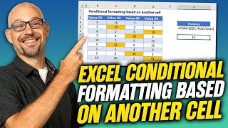
In this video see how to color a row with conditional formatting using an Array Formula & the MATCH Function that will lookup Two Lookup Values in a corresponding Table.


What a great video, Mike, I have never imagined to concatenate cells with Match function. Thank you so much!!
You are welcome so much!!! Yes Indeed, Concatenate and it becomes one value that MATCH can read : ) Thanks for the support, aguerojg, with your comment, Thumbs Up and Sub : )
Nice video bro..I have been watching your videos last 2.6 year...You always rock
Thanks for watching for 2.6 years, Deepak!!! Thank you for the support with your comment, Thumbs Up and Sub : )
This was a live-saver! I do inventory and I have an Excel map of all the warehouse buildings and racks. I wanted to input an item number, have it search inventory records, and highlight on the map everywhere in the building that item is stored. Took some finagling but it works like a charm. I had to use a helper TRUE/FALSE column, but maybe I can integrate it.
Your welcome Mike, thanks for your great channel I find the answers to a lot of problems I think I should call you a teacher
That is what i do for a living - I am a teacher : ) Glad we are hanging out here on our Online Excel Team!!!
I really was looking for this Mr. Mike thank u so much i really appreciate
You are so much welcome, Ismail!!!!! Thank you very much for your support!!
Thanks Mike. Just Love Array Formulas. :)
You are welcome, John!!!! Me too - I love Array Formulas : )
Hi, thanks for the video. I have a question, can you conditionally format merged rows dependent on the text values of another cell?
Thanks Mike for this EXCELlent video
You are welcome, Syed : ) : ) : )
That was revision of funwith excel... Good one mike
I am not sure what you mean, RRR, but thanks for watching : )
Great video as always!
Thanks, as always, Teammate : )
Great trick...hopefully it works good and quick in big data
I do not think so - cuz it is running an array calculation in each cell, and MATCH is doing Exact Match and because Conditional Formatting is Volatile and calculates often. BUT, if it is on the Lookup Table side, where the table is probably small, it should be OKAY... Thanks for the support, NoShadowOfDoubt : )
Fully aware about CSE in cells. Completely unaware of the "don't use CSE in Conditional Formatting"... until now.
Thank you for upping my Excelfu.
You are welcome for upping your Excel Fun, Rich!!! Thanks for your support with your comment, Thumbs Up and Sub : )
Done and Done. Thanks.
Thank you, thank you, thank you, Rich : )
wow! I was going to write a formula in condition formatting that highlight duplicates based on 2 columns. I haven't even started yet when you uploaded your film. And now I know I will use your brilliant solution in mine. Thank's Mike!
Wow, Teammate : ) But, wait... "Are Two Combined Values in a Different List?" and "Highlight Duplicates?" are different questions and formulas... How can you use my solution?
One list, I forgot to write :). I'm gonna combine it with ROWS: MATCH($A5&$B5;$A$4:$A5&$B$4:$B5;0)-1
I am not sure, can you e-mail me the Excel Workbook so I can take a look, to: excelisfun at gmail. : )
Done :)
For Conditional Formatting the Row with a test whether or not two items are in a row to see if there are duplicates, I think this is more efficient: =COUNTIFS($A$5:$A5,$A5,$B$5:$B5,$B5)>1 than a formula like this: =MATCH($A5&$B5,$A$4:$A5&$B$4:$B5,0)-1
Thanks for fun with array :-)))
You are welcome, Most Amazing Teammate Bill "billszysz.com" Szysz!!!! : ) P.S... Can't wait : ) : ) : )
Great video Mike :-)
Glad it is great for you, K B!!!! thank you for watching, having fun and supporting excelisfun : )
Thankssssss mike
You are welccccccommmmmmmmmme, Mohamed!!!!! Thanks for your support : )
Amazing ..
Glad it is amazing for you, Bindhyesh! Thanks for watching, and thanks for the support with your comment, Thumbs Up and Sub : )
It is fun watching that subscribed number growing. I wonder what the rate of growth is?
Thanks for watching the videos and the subscriber growth, Dae H!!!! The growth rate is actually very small in terms of many other of my RUclips Channel Friends like ruclips.net/channel/UCuGn3ioftOo6jvHE1YK4Bfw, ruclips.net/user/IGNentertainment and others. I have worked every day for over 10 years giving away free education that included videos, Excel Files, pdf Notes, Practice Problems and more; and I am still stuck at under 1/2 million subscribers. What confuses me is that the demand for Excel skills & Excel Training is massive, huge and world wide, but no matter what marketing and promotion endeavors that I try, I can't seem to match this supply of free Excel education here at the excelisfun Channel to the demand for Excel Training that is out there. I just wish I could find the magic recipe to help give away the content of this channel to more people in the world : )
Mike, I was wondering how VBA macro recorder handles the keystrokes of C+S+E & curly brackets?
When you use the Macro Recorder to enter a non Ctrl+Shift+Enter Formula the recorder uses the command ""FormulaR1C1". When you use the Macro Recorder to enter a Ctrl+Shift+Enter Formula the recorder uses the command "FormulaArray". For example:
ActiveCell.FormulaR1C1 = "=SUM(R[-18]C[1]:R[-12]C[1])"
Range("I55").Select
Selection.FormulaArray = "=SUM(R[-19]C[2]:R[-13]C[2]*R[-19]C[1]:R[-13]C[1])"
See, I told you you are great!
Just keep clicking that Thumbs Up, commenting and tell all your friends to come have fun with us at excelisfun channel here at RUclips : )
Very good video. Can we join MATCH with IFERROR here? But anyway if conditional formatting is taking care without using IFERROR, then nothing like it. Thanks for uploading :)
In a cell you would not want to use IFERROR; if you are checking to see if the items are in the other lists, then you would use ISNUMBER around MATCH. Anyway, no need to use either in the Conditional Formatting dialog box : )
I would like highlight the NON-Match cell, how to do this ? Thank you
Great!
Glad it is great for you, Sandeep!!!! Thank you for the support with your comment, Thumbs Up and Sub : )
Welcome Mike. It is always encouraging to hear from you. Your videos & companion materials are splendid.
We do have splendid fun with our Online Excel Team!!!!
Yes Mike, I can see that.
Go Team!!!!!
👍👍👍👍👍
good godd
Is there a way to use the similar formula-way to do the icon sets? For example, based on the quantity of products being sold, when a particular product been sold more than x numbers, show Red light icon, between x and Y numbers, show Yellow light icon, and less than Y number, show Green light icon...etc. or based on the product selling price ...etc.
or maybe we can use the "KPI" in the PowerPivot data model to do that?
Yes, that can be done. Just use the built in options: Conditional Formatting, Highlight Cell Rules, and then use the Between, less than and Great than options. You can add multiple Conditional Formatting Rules to the same range. I have many video on these topics. Here is one: ruclips.net/video/GRfe4bHsjhI/видео.html
Thank you...
How can count background specfic text mean if i put in yellow colour 20. All yellow in 20 then green 50 after i want count 50 with green color how many and 20 yellow how many i think you understand what i want thanks so much
I do not know. I am sorry about this. You can try this great Excel Question site: mrexcel.com/forum
Ha ha ha, for the first time I'm the number "one" viewing your video
Thanks for being #1 and for your support, Digital Cooking : )
I actually saw the notification but I was busy watching his other excel video. No fair, haha.
Two at once, nice!!!!
Hi friend 👋,Comment is funny hahaha
Will u teach macro please?
I am no good with writing VBA. I have some basic videos on Macros, but it is better to learn VBA from other people like these RUclips Channels:|
ruclips.net/channel/UC-vzNYU9x8IYPk_r89mGvXA
ruclips.net/channel/UC9OIUFZfYqELCFwWxT7OpKQ
ExcelIsFun thank you for the recommendation!
Hello, subscribed to these lessons a few years ago.I got emails on a regularly for a while the then all of a sudden It stopped and I've not received any email ever since.
I do not know what has happened. I e-mailed RUclips about this, but they do not answer. The best thing for you would be to use the Bell Icon next to the Subscribe button to get notifications that way. Can you try to do that and get back to me and see if that works?
Strange how it interprets those the way it does. I thought you were going to have to use ISNUMBER.
It has been like that always. Most do not know, though. But now we do!!!! : ) Thanks for the support, Jason M!!