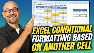
Conditional Formatting based on another cell | Google Sheets

Поделиться
HTML-код
  • Опубликовано: 3 фев 2020
  • Conditional Formatting in Google sheets is one of the few things that limits you a bit - at least when compared to Microsoft Excel. That is, unless you know all the ins and outs of advanced conditional formatting in Google Sheets. In this video, I'll teach you:
    • Quickly how to format one cell based on what is in that same cell
    • How to format an entire row of cells based on text in one cell
    Here are some other videos you might like:
    • • VLOOKUP In Google Shee...
    • • Pivot Tables in Google...
    Thanks again for watching. Stay tuned for my next video coming out next week. If you would, please help to promote my channel by subscribing and clicking the bell notification. Or at least hitting the like button. Also, feel free to comment on the video - good or bad. I'm in it to learn as well!

Комментарии • 98

  • @LadyHawke904
    @LadyHawke904 3 года назад +7

    I am learning google sheets for my own personal use and your videos are easy to understand and encouraging. I appreciate that you generally focus on one formula or action per video. Thank you.

  • @harrisongraceacademy
    @harrisongraceacademy Год назад

    This video helped me immensely! Creating a sheet to tally attendance, wanted to have the "name" column change colors based on if the required events were attended. Used a countif in a different column to tally attendance and used your video to change the color based on that value. thanks a ton!

  • @thedarkarmy0109
    @thedarkarmy0109 2 года назад

    I've learning so much things from this short video, well done mate!

  • @countmoney7
    @countmoney7 2 года назад

    I was working a ToDo list and Camping Packing list that would strike through the item in the cell when a checkbox was changed too TRUE. Nailed it! Your video was quick and just what I needed. Now when the checkbox is clicked that cell changes color and the text in the adjoining cell gets struck through...just like a my old fashioned hand written lists. Now my girlfriend and I share lists on our iPhones/iPads and when one of us completes a task or verifies we have packed an item the other can easily see it so we don't do things redundantly or forget something altogether. Much appreciated!!

  • @acemakerjay
    @acemakerjay 2 года назад

    I've been watching all your Google Sheet videos and they are extremely helpful. I'll be sharing them with friends and family. I think I can use this for attendance records.

  • @sithwarrior
    @sithwarrior 2 года назад

    I use Sheets for maintain a game collection of Digital, physical and free games given with subs, you showing how to move the position of the formulas to show which one has preference was a big help since I couldn't figure that out (which kills me how dead simple it is to move them around lol)

  • @YePainLab
    @YePainLab Год назад

    So much better than the google sheets help site! Using this to keep track of daily word count goals. Thank you

  • @philzills8219
    @philzills8219 3 месяца назад

    Thank you for putting these videos together. I have found them very useful in completing a multitude of tasks.

  • @erichepperlewp
    @erichepperlewp 6 месяцев назад

    This is the #holyGrail of Google Sheets, bro! You make it so simple to understand. Changing a whole row based on the contents of a cell in that row is something I find myself having to often. I am bookmarking this

  • @MalNoorulbari
    @MalNoorulbari Год назад

    It helped a lot, thank you very much!

  • @TomGarland
    @TomGarland 4 года назад +1

    Thanks! That helped a lot!

  • @yasa.42
    @yasa.42 2 года назад

    Solved my issue. Thanks

  • @strawberry__icecream
    @strawberry__icecream 5 месяцев назад

    awesome, tutorial

  • @pj04laus
    @pj04laus Год назад

    Thank You So Much! 😁

  • @kimlirit3710
    @kimlirit3710 2 года назад

    Hello! I would like to highlight a cell range and remove the highlight once a text in a certain cell appears. Would it work on your sample? Appreciate your help. Thanks in advance!

  • @trinicebowens8329
    @trinicebowens8329 3 года назад +2

    I am using this video to (hopefully) create digital assignments for my 6th grade math students.

  • @SteadyForceSolutions
    @SteadyForceSolutions Год назад

    Great video. would love to see a video on how to to conditional formatting based on the percentage of a number in a different cell. Example: Goal Tracker spreadsheet: Goal Sell 100 pens per week. and in subsequent cells we add weekly sales updates. Cell A1: 100, Cell B1: 90, C1: 100, D1: 75, etc. Then the conditional formatting shows a colored background based on level of success. 0% achieved, or 0 sold in this scenario is red, 100% achieved or any sales 100 or more is Green. the cells would shift from red to green as you reach your goal each tracked week.
    High quality stuff here though. tag me if you create this video!

  • @teddiebrune4068
    @teddiebrune4068 3 месяца назад

    Thank you!!!

  • @jasunlg
    @jasunlg Год назад

    That was great, thank you for this information.

  • @bluething3D
    @bluething3D Месяц назад

    Thanks! I'm setting up a project tracker for developing a video game.

  • @Blenda73
    @Blenda73 3 года назад

    Excellent video. I am trying to highlight a cell when someone makes a change. I am sending a sheet to about 8 people for their updates and I want to track them. Is there a way to use conditional formatting to color a cell when it is changed?

  • @Billyonaire__
    @Billyonaire__ 2 месяца назад

    G, great video

  • @shivaraj108
    @shivaraj108 Год назад +1

    Great video thanks. Is it possible to format one cell based on anther cell equaling a DATE? Any date, i.e. if the other cell has text or formula than no format but if a date is entered then it changes color? Thanks for your consideration. ANSER FOUND: =isdate(B2) Where B2 is the cell with the referenced date

  • @user-nz7ld7qg2o
    @user-nz7ld7qg2o Год назад

    Can this be done to change the color of a cell based on if its value is , or = another cell? I am wanting to use the sum at the bottom of a column to compare it to a target number in another cell and each cell change based on the comparison to the other. For example if A4 is > G18 then both cells would turn red to indicate that the target number has not been reached but it would change to green when they are equal based on the sum of the column G.

  • @soglobal7637
    @soglobal7637 3 года назад +1

    Hi.. liked yr video & you hv great explanation skills. Bravo!
    I hv a specific question.. pls if you can resolve for me..
    There is set a transactions on my googlesheet and need to highlight the rows which have Unpaid Bills. The particular Cell (Payment value Cell) has three scenarios:
    1. Empty - bill unpaid - the entire row to be highlighted in Red
    2. Payment value Cell - Value is equal to Invoice value (This value is already in next Cell - same row) then No colour - non highlighted.
    3. Part payment - if Cell Payment Cell is less than Invoice value - then entire row must be highlighted in Yellow.
    Hope you got it.
    Thks!

  • @4444hash
    @4444hash 3 года назад +1

    Hi. New subscriber here. Im just curious if it is possible to put a automatically put the date today when I click on another cell. Because I use sheets for studying. For example I clicked A2, A1 will show the date when I last edited or click. What I do now is manually putting dates to track when I last studied a specific row. Thank you.

  • @fatimagajia4823
    @fatimagajia4823 3 года назад

    Hi I am trying to to use a combination of conditional formatting and "blank" cell, but i just cannot find how to do that anywhere.
    eg=NETWORKDAYS(B3,C3,Holidays!C59:C67) i have this formula to calculate how many days from one date to another, then adjacent to that column i have this formula
    =NETWORKDAYS($B3,$A$1,Holidays!C60:C68) to show how many days it has been in real time.
    This is where it becomes tricky, the next column i enter an end date but the clock keeps on ticking.
    I want the clock to stop and the cell to go Blank, when i add the end date.
    Do you have any ideas?

  • @MarkT923
    @MarkT923 4 года назад +1

    Just tried following your steps and it's still not working on my end. Not sure if I'm doing something wrong. I'm trying to have a cell highlight a specific color when the next cell over has text inputted in. For example, I'm trying to highlight cell G23 in green when cell H23 has the word "Yes" inputted in. Any help will be appreciated. Great work with the video. I just subscribed!

    • @whyworksmarternotharder
      @whyworksmarternotharder  4 года назад +1

      Sorry for the delay. Ensure you have the dollar sign in the right spot. Watch again at the 3:00 mark

  • @bronfoth
    @bronfoth Год назад

    I am learning Google Sheets/Excel for a variety of uses for research and data management uses for private investigation work. I use a mobile device for most of my work so it's extra tricky

  • @gerardomejiaenciso2717
    @gerardomejiaenciso2717 3 года назад +1

    Hi! You helped me a lot, but I have a question. You said in your formula that the name would become red if no text was in certain cell, which was translated as "=C4="" (the quote marks empty because cell is blank) but what happens if I want it to change the name to green by adding any text? What do you need to include in the formula between the quote marks to indicate that any text written in there will affect the other cell's color?
    I don't know if I explained myself properly.

    • @TheOgi22
      @TheOgi22 2 года назад

      You described it correctly.
      I'm looking for exactly the same.
      ruclips.net/video/xqhqtxAWjgo/видео.html&lc=Ugyj_I1LzX-DO-A_agd4AaABAg

    • @TheOgi22
      @TheOgi22 2 года назад

      Edit:
      I find it:
      =$A1>0

    • @TheOgi22
      @TheOgi22 2 года назад +1

      Edit2:
      I think this entry is more correct
      =$A1""

  • @InnerProp
    @InnerProp 4 года назад +1

    I'm trying to track my weight. I want the conditional format to be green if the weight is less than the last recorded weight and red if more than the last date. I did it for the second weight, but when I tried to copy it down for the rest of the month it only compared every weight entered by the first weight.
    How do you set it up with relative references? Alternatively, how to you copy and paste conditional formatting?

  • @cuisinera4307
    @cuisinera4307 2 года назад

    thanks

  • @PCITV
    @PCITV Год назад

    Great video! Thank You. I would like to change the text in one cell based on the value in another cell. For example, I have used the formula =IF(E6

  • @BigIsleJ
    @BigIsleJ 3 года назад +1

    Thanks

  • @virginiasmall6420
    @virginiasmall6420 2 года назад

    I am constantly trying to turn a value red if another value equals something. Like if I used a credit card in my budget I want the amount I spent to show up red. I'm loving your videos, so easy to go down the rabit hole. . . I think I'm about 5 videos away from where I started with one of the budget videos.

  • @Reflexiones101
    @Reflexiones101 Год назад

    I have a sheet with data of 20 players where the players data is given one after the other, but separed by players in the same column and I want to highlight in different shades of green the 3 highest in investments, the 3 highest in net Value etc in Google drive, how do I do that?

  • @mommasa1
    @mommasa1 3 года назад +1

    Is it possible to do this across sheets? Or use a control tab to format information?

    • @whyworksmarternotharder
      @whyworksmarternotharder  3 года назад

      Not sure I completely understand the question. What is it that you’re trying to accomplish?

    • @kerjasampinganku
      @kerjasampinganku 3 года назад

      I found this useful, may can relate: Create an Event Reminder use Color | Status: Finish; Today; Three Days Until 1 Day Before Event ruclips.net/video/7FdByf2TEo0/видео.html

  • @marks3541
    @marks3541 2 года назад

    Was wondering if you had a values in column B and you had a vlookup placing values in cells column C. How can you conditionally format if B2 doesn't equal C2, and B3 doesn't equal C3. When value in rows in c doesn't match the values in Column b then I should see cells in column C highlighted. IF #NA appears in Column C that should also be considered as not matching.

  • @JulioPereira-xc8qv
    @JulioPereira-xc8qv 10 месяцев назад

    Brother I want to make a Vlookup cell copy the same fill as the cell to the left... is that possible?

  • @zedestatebc4437
    @zedestatebc4437 Год назад

    How about if we want a row to be highlighted if a cell specific cell is populated with anything. What would be the customized formula?

  • @EamonKelly
    @EamonKelly 2 года назад

    Is there a formula that can change the color of a row if a particular cell is blank?

  • @gauravarchy
    @gauravarchy 3 месяца назад

    can any one help me on removing conditional formatting in a selected range where canditional formatting is applied/

  • @sexybandboy
    @sexybandboy 4 месяца назад

    THANK YOU SO MUCH!!!

  • @WenSaiPanther
    @WenSaiPanther 21 день назад

    Hi. My goal is to find a way to copy a cell and text color to copy the origination of a cell's and text's colors. For example, cell a2 has the word "completed" and the text is bold red with the cell's color purple. When I type "completed" in cell c35, it automatically makes that cell's color purple, and the word becomes bold and red.
    How can I do that without a script?

  • @foreverpeacefulevents1146
    @foreverpeacefulevents1146 Год назад

    I have watched a few videos on conditional formatting in hopes of what i am looking for! But I cant see to find it :(
    I have a drop down menu (yes, no and pending) in column "B" and in column "A" I want it to reflect the number "0" when "No" is selected. How do I do this?! Am I researching the wrong equation? Ha! Thank you!

    • @whyworksmarternotharder
      @whyworksmarternotharder  Год назад

      You are going to want to check out the if formula ruclips.net/video/Co3aI2Jq-Yw/видео.html

  • @lauyunhong4499
    @lauyunhong4499 2 месяца назад

    Hi, i want to ask that the symbol for empty is "". Then how about not empty? What is the symbol for not empty in google formula

  • @pfnichols
    @pfnichols Год назад

    How can I conditionally format a cell based on whether or not it is < than or = to the average of a range of cells?

  • @sunkidibali7080
    @sunkidibali7080 Год назад

    how can i copy characters from a cell to another cell as a result of a check list ?
    \

  • @jamhurdavronov
    @jamhurdavronov 2 года назад

    on my google sheets i don't know how this happing: row6 and 7 color keep changing to white i change back to black and if you go to next column it again writing white: is there any solution PLEASE

  • @TheOgi22
    @TheOgi22 2 года назад +1

    Hello.
    How to color the whole row if the first cell is not empty?
    I don't know how to enter the formula.
    Is there documentation?
    Edit:
    I find it:
    =$A1>0
    Edit2:
    I think this entry is more correct
    =$A1""

  • @warddepoortere1264
    @warddepoortere1264 3 года назад +2

    Thank you for the explanation.
    But it doesn't solve my problem. I'm using Google sheets for excercises accounting for my high school students. In stead of having to correct each excercise manually, I want to use a kind of autocorrection. I want to complete each excercise with a sheet in which I can copy the correct solution. When this is done, cells in the solution of the students which aren't correct, should light up in red.
    But is more complex than that. In accountancy it doesn't matter if A proceeds B: when B proceeds A the solution can also be correct. But in my solution I might have A proceeds B and the student can have B proceeds A. In that case the cells would lighten up red, while the students solution is still correct.
    Can you help me out?

    • @whyworksmarternotharder
      @whyworksmarternotharder  3 года назад

      I think you need to use a combination of an if statement and then combine that with conditional formatting. I’d check out my if video.

    • @warddepoortere1264
      @warddepoortere1264 3 года назад

      @@whyworksmarternotharder Thank you

  • @1-vybz
    @1-vybz 2 года назад

    When a date is input into a cell, Iwould like to use conditional formating to change the colour of another cell within a calender so that it highlighted. Any help/advice would be welcomed.
    Thanks

    • @whyworksmarternotharder
      @whyworksmarternotharder  2 года назад +1

      ruclips.net/video/H1bEpd-i4DM/видео.html

    • @1-vybz
      @1-vybz 2 года назад

      @@whyworksmarternotharder Thanks very much. I'll have a look at it now.
      Super

    • @1-vybz
      @1-vybz 2 года назад

      @@whyworksmarternotharder Thanks for the video but its not quiet what Im after.
      I have a calender which extends over a 5yr period. I would like the calender to be dynamic in that I have a series of dates (associated to tasks) which when input into an adjacent colum I would like the cell in the calender of that date to be highlighted.
      Any ideas how I could so this?

  • @Saint_Ale
    @Saint_Ale 5 месяцев назад

    Is it possible to also have the gmail/name of the person populate when they click a checkbox?

  • @nepdelosreyes
    @nepdelosreyes 4 года назад +1

    How do you highlight a cell if another cell does not have the data you typed/chose?

    • @whyworksmarternotharder
      @whyworksmarternotharder  4 года назад

      Not sure I understand your question. Can you give an example or explain further?

  • @KingXamer
    @KingXamer Год назад

    GG BRO

  • @lelelulu7836
    @lelelulu7836 10 месяцев назад

    can "true" or "false" condition change to any date? i mean the cell turn yellow when u put any date.

  • @hazenstribling2646
    @hazenstribling2646 13 дней назад

    Do you know of any way to determine the VALUE of one cell based on the color of a different cell?

  • @attaqkhq6432
    @attaqkhq6432 Год назад

    I am tracking monthly income. I would like for cell B2 to turn green if it is greater than B3 and red if it is less than B3. Any idea how to do this?
    And then, I would like for B3 to do the same based on the value of B4. And for B4 to change based on B5, etc.

  • @anowar77
    @anowar77 2 года назад

    i need to change color based on another cell if is not empty

  • @jenpeak7005
    @jenpeak7005 3 месяца назад

    trying to figure out how to use condtional fromattin gwith a drop down

  • @shelleyleahy593
    @shelleyleahy593 2 года назад

    Trying to have more than one condition to drive COLOUR coding per row

  • @gustersavon
    @gustersavon Год назад

    I used this to better format my grades

  • @mikewilson946
    @mikewilson946 2 года назад

    How do I turn a cell the same color as another cell just based on the fill color of the reference cell, NOT the value inside the cell?

  • @christopherc9935
    @christopherc9935 2 года назад

    I want to conditionally format a cell become a certain color when a currency value is added to another cell in the same row

  • @MasterGator4
    @MasterGator4 Год назад

    Setting up a fantasy hockey sheet and trying to make a group of cells to turn red if a teams budget in a certain department ($10,000,000)
    For some reason there's 3 cells that just won't change color like they should. Just a glitch, or am I doing something wrong?
    Formula I used was...
    =G153

  • @nickcavolli3072
    @nickcavolli3072 2 года назад

    I want to conditional format text populating based off Yes or No dropdowns. No luck so far

  • @TheJakeThatVlogs
    @TheJakeThatVlogs 3 года назад

    I want a cell to change color if a different cell has content in it

  • @eplaygaming1
    @eplaygaming1 5 месяцев назад

    I'm needing to change colour of number based on value of cell above. IE number in A3 is lower than A2 (make red) if higher turn blue.
    Its easy in excel, but Sheets has me stumped. 😅

  • @carriebrooks8293
    @carriebrooks8293 4 месяца назад

    I followed the steps meticulously, but even with the dollar sign in the formula and the rule at the top of the list, the row is not changing color! Help!

  • @kevincrandall2751
    @kevincrandall2751 9 месяцев назад +1

    You get five seconds then I'm on the next video

  • @timelesstimesgoneby
    @timelesstimesgoneby 2 года назад

    Do you have Facebook so I can send what I’m looking for to do

  • @patricksexton1501
    @patricksexton1501 11 месяцев назад

    Good videos and thank you for your content. But, what's with the intro music always being 3 times the volume, I have to turn you up to hear you and then I worry my speakers are going to blow when your intro music plays.

  • @PistolaMasajeadora
    @PistolaMasajeadora Год назад

    didnt work for me :(

  • @JanetCunningham-ix8of
    @JanetCunningham-ix8of Год назад

    Statement spread sheet. If balance is positive positive State: "Balance on account". If balance is negative State: "Balance due".

  • @JulioPereira-xc8qv
    @JulioPereira-xc8qv 10 месяцев назад

    Video once a week but you only have 30 videos :(