6.7. Actuarial Math: Life Insurance Benefits G

Variable insurance benefits when payments are made at end of year of death (discrete)
Typos:
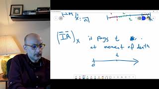
At 5:15 in (IA)x:angle_n, there should be a small (1) on top of x to indicate it is term benefit.
At 30:28 please add 2 and 3 to the second and third term. so the equation should be:
E[Z] = 100000 [v(.02) + 2 (v^2)(0.98)(0.04) + 3 (v^3)(0.98)(0.96)(0.06)] = $23644.

[@joeytan9995]

Thank you Dr. for the clearly explained video!! Your videos is so helpful to my actuarial science course I'm taking right now

[@DrAmjadRabi]

Many thanks and all best wishes in your study

[@IOnlyPlayRs]

I wish I found your videos earlier! Thank you for putting this entire series on RUclips.

[@DrAmjadRabi]

My pleasure. thank you

[@DrAmjadRabi]

Typos:
- At 5:15​ in (IA)x:angle_n, there should be a small (1) on top of x to indicate it is term benefit.
- At 30:28​ please add 2 and 3 to the second and third term. so the equation should be:
E[Z] = 100000 [v(.02) + 2 (v^2)(0.98)(0.04) + 3 (v^3)(0.98)(0.96)(0.06)] = $23644.

[@anisamalik8854]

Hi at 30:45, how did you get that equation for the expected value of Z?

[@DrAmjadRabi]

in the description under each video (and also as a comment as well), i added corrections for some typos. Please take note of them. For this, please add 2 and 3 to the second and third term. so the equation should be:
E[Z] = 100000 [v(.02) + 2 (v^2)(0.98)(0.04) + 3 (v^3)(0.98)(0.96)(0.06)] = $23644.

[@anisamalik8854]

@@DrAmjadRabi aaah thank you! But I’m not sure how you got the general formula tho?

[@DrAmjadRabi]

@@anisamalik8854 i see. I think you need to review the first few vides on review of probability theory to refresh on how to calculate the expected value (expected value of a RV is the weighted average of all possible values of the variable. The weight here means the probability of the random variable taking a specific value). Here it is a simple calculation of the APV (review also first introduction video to remind yourself on the difference between PV and APV). So for each outcome possible (the three different payments discounted back to time zero), you need to multiply it with the specific probability for that outcome to occur, and then sum up to get the expected value. Again, this is built on earlier material. I encourage you to watch the videos in order as concept built on each other.

[@flyinghos]

Thank you always for the great content. As for the relationship with A35:(1) = v*q35 + v*p35 = v, would this hold for Ax:n as well? Such that Ax:n = v^n (since Ax:n = v^n * nqx + v^n * npx)?