Lecture 14 - Support Vector Machines

HTML-код
- Опубликовано: 8 сен 2024
- Support Vector Machines - One of the most successful learning algorithms; getting a complex model at the price of a simple one. Lecture 14 of 18 of Caltech's Machine Learning Course - CS 156 by Professor Yaser Abu-Mostafa. View course materials in iTunes U Course App - itunes.apple.c... and on the course website - work.caltech.ed...
Produced in association with Caltech Academic Media Technologies under the Attribution-NonCommercial-NoDerivs Creative Commons License (CC BY-NC-ND). To learn more about this license, creativecommons...
This lecture was recorded on May 17, 2012, in Hameetman Auditorium at Caltech, Pasadena, CA, USA.


Amazing how you unravel it , like a movie , the element of suspense , a preview and a resolution.
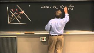
Hit the like button when he explains why w is perpendicular to the plane. Great detail in such an advanced topic!
Wow! this is the best explanation to SVM's by far I've come across, with right mathematical rigor, lucid concepts and structured analytical thinking put's up a good framework to understanding this complex model in a fun and intuitive way.
Agreed. The MIT one is not as good as this one since the MIT professor did not tie ||w|| to margin size via geometrical interpretation as this vdo does (he chose to represent w wrt. the origin, which is not a very meaningful approach). The proof of SVM in this vdo is much more geometrically sound.
What a charming prof. Like his teaching style. Thank you Caltech for sharing this
I am amazed to see how smart the students are, understanding the whole ting in 1 go and actually challenging the theory by putting forth cases where it might not work.
This is the best (most geometrically intuitive) SVM lecture I have found so far. Thank you!
This is the most in-depth explanation of SVM in RUclips. Very juicy
Thanks Dr\ Yasser ,you are honor for every Egyptian
Actually, he's an honor for every human being. People like him should makes every human being proud of being human.
writing my bachelors thesis about SVMs atm. it's a great introduction and very helpful for understanding the main issues in a short time. Thankyou!
I watched almost all the SVM from youtbe and I got to say, this one for me was the most complete
I haven't watched this one yet, but same i have watched so many vids and still dont totally get the ideas
This lecture is sooo good! One of the cool things is that people here don't assume that you know everything unlike so many other places where they expect that you know about the basic concepts of optimisation and machine learning!
best explanation on you tube. No other lecture provides mathematical and conceptual clarity in SVM to this level..Bravo :)
people like you save my life :)
Absolutely well done and definitely keep it up!!! 👍👍👍👍👍
Great Prof. Step by step explanation is amazing
In sovjet rashiya, machine vector supports you.
this is not a sovjet rashiya accent
Really helpful explanation..got what SVM is..Thank you so much professor!
this is the best lecture explaining SVM. thank you Professor Yaser Abu-Mostafa
The best SVM lecture I've came across. Thank you for sharing this!
I rewinded this a number of times and i finally got it. really well explained!!
such a gentle man and inteligent Professor.
I bow to your teaching _/\_. Thank you.
from 12:15
It means that you extended the features X with 1 and weights W with b as in perceptron.
And these extensions are removed from X and W after normalization.
very good point, if it helps anyone have a look at augmented vector notation and it should clarify what he means
seriously dude this is awesome.. after many attempts finally I understand the SVM..
The best explanation to the SVM
I loved loved loved all the lectures , you are an amazing professor !!!!
If you understood this lecture and if you are the girl on your profile picture, I would like to be friends.
Just kidding :)
^creepy internet loser detected
Bravo Dr. Yaser, excellent explanation! Now looking forward Kernel Methods lecture :)
One of the best machine learning lecture. I would like to know.
How to solve quadratric programming analytically. So that the whole process of getting hyperplane can be done analytically.
Thank you very much for the best lecture on SVM in the world. Probably, Vapnik himself would be able to teach/deliver the SVM clearly as you do.
Nice, clean presentation.
"I can kill +b"
38:02
at 34:29, Observe closely, When Prof. Yaser is explaining the constrained optimization, there is an background music as his hand moves. "Boshooom"... ! It just sounds so natural, as if Prof. Did it !
Thank you for sharing this. So helpful :)
This explanation is really great. However, much more intuitive and better developed is the one in the Machine Learning course by Columbia University NY in EdX.org. It worthy to revise it.
Thank you for the lecture Professor!
What a class. Thank you caltech
Best explanation ever! thank you
your lecture cannot say about it less than amazing...Thank you so much...
This is a very well produced lecture. Thank you for sharing. :)
How simply you explain things. Wonder I can explain complex things like you do.
really nice video...understood SVM at last :)
Woww, man this amazing.
Thank you sir! BTW, I would have applauded at this moment of the lecture: 22:37
Thanks a lot, very well explained!
The intuition is GREAT! Thx!
Summarized question: Why are we maximizing L w.r.t. alpha at 39:25?
Slide13 at 36:06: At extrema of L(w,b,alpha), dL/db=dL/dw=0, giving us w =sum(an*yn*xn) and sum(an*yn)=0. These substitutions make L(w,b,a)=L(alpha) in the slide 14 = extrema of L. Then why are we maximizing this w.r.t alpha?? He said something about that in slide 13 at 33:40, but I could not understand. Can anybody care to explain?
***** The are two terms (t1, t2) in the equation. Generally, The minimum of the first or second term is what we don't want. Hence we maximize alpha to reach a point in t1 and t2 where both of them meet which ensures the equation (t1+t2) is minimized.
The reason to max alpha is related to KKT method that you can explore. Put it simply, when you have E = f(x) and constraint h(x)=0. To optimize min_x E with the constraint is equivalent to optimize min_x max_a L. The reason is, since h(x)=0, then if you can find a solution x satisfying the constraints, you must have max_a a*h(x) = 0. Hence max_a L = max_a f(x)+a*h(x) = f(x), and min_x max_a L = min_x f(x) = min_x E. This is the conclusion.
To further explain, since for a solution xs, you have max_a a*h(xs) = 0, a natural result is, either you have h(xs) = 0, or you have a = 0. The former, h(xs) = 0, means a != 0, further means you find the solution xs by using a. The latter, a = 0, means your solution xs solved by min_a E already satisfies the constraint h(xs)
I salute you Sir!. What a great way of teaching! I think, I understood most by just one viewing of these lectures.
Do you teach any other courses? Can you put them on youtube also?
Watched a video on Lagrange Multipliers and now Im back again.
24:48 why isn’t maximizing 1/||w|| just simply minimizing ||w||, why did we make it a quadratic; wouldn’t that change the extremums?
Thank you very much for sharing these wonderful lectures! I have some thoughts about the margin. It seems, that start of the PLA with weights defining the hyperplane placed between the two centers of mass of data points is better to achieve the maximum margin, than the start with all-zero weights. Let R1 and R2 be the centers of mass of data points of the "+1" and "-1" categories, respectively. Then the normal vector of the hyperplane is equal to R1 - R2 (direction is important) and the bias vector is equal to (R1 + R2)/2. Thereby, the vector part of the weights is initialized as w = R1-R2 and the scalar part as wo = -(R1-R2, R1+R2)/2 (the inner product of the normal and bias vector multiplied by -1).
this is the harder course for the moment
I haven't fully understand the math derivation. will come back to it soon:)
This is really very nice and helpful in my research work. I would have love to know more about the heuristics you talked about for handling large dataset with SVM
Wow, this is brilliant.
Very nice presentation.
Thank you a lot
Un mot merveilleux...
Well explained! Thanks a lot!
10/10 would listen again
I have some questions:
1. in slide 6 at 13:53, I still don't understand the reason behind changing the inequation into equal 1. the professor just said so that we can restrict the way we choose w and the math will become friendly. but is there any other reason behind this? like, can we actually choose any number other than one, maybe equal 2 or equal 0.5? seems both of them will also restrict the way we choose w
2. in slide 9 at 24:56, why maximize 1/||w|| is equivalent to minimize 1/2 wt w? any math derivation behind this? because I think I don't get it at all
any answer will be appreciated
Maybe this lecture can give a full intuitive explain of your question. ruclips.net/video/_PwhiWxHK8o/видео.html
1. in slide 6 at 13:53, That expression is the distance between any x point and vector w. We just arbitrarily set that if only the distance is bigger than 1, x can be regarded as a positive example. So the number 1 is just a trick to let formula more easy to optimize.
2. max( 1 / ||w|| ) → min( || w| | )→ min( || w|| ) → min( squree( || w|| ) ) → min( squree( wtw ) ) → min( squree( wtw ) / 2 )
Why there is a `2` is that when you take the derivatieve of squree( wtw ) in the next step, and the constan 2 will be canceled by the result of derivative.
Very helpful !.. thanks a lot
Thank you very much, very helpful !
Excellent lecture
I love his accent! :)
arabic accent
@@spartacusche Yeah probably Syrian :D
@@Hajjat No he is from Egypt
In the constraint condition of |w^T.xn +b| >=1 how is it guaranteed that for the nearest xn, the |w^T.xn +b| will be 1 ?
you can scale the hyperplane parameters w and b relative to the training samples x1,...,xn. (note that w doesn't have to be a normalised vector in this case and as a result the term | +b| gives not neccessarily the euclidean distance of sample point xn to the hyperplane) you have to distinguish between the so called functional margin and geometric margin (see f.ex. Christianini et. al). you just want the hyperplane to be a canonical hyperplane. so you can choose w and b so that xn is the sample for which the condition | +b| =1 is true and for all other samples xi the value of |+b| is not lower than one. note that there exists another support vector xk (with an opposite class label) for which the value of |+b| =1, as the hyperplane is defined via at least 2 samples which have the same minimal distance to the hyperplane. all of that states on the fact that the hyperplane {x|+b=0} equals to {x|+cw=0} for an arbitrary scalar c (it is scale-invariant) hope it was useful!
Please see my reply above to +Vedhas Pandit. It is because, when you find a solution x_n with KKT method that meets the constraint, you either have alpha_n = 0 (for interior points x_n), or the solution x_n is on the boundary of the constraint, i.e., |wx+b| = 1.
For those watching this lecture at 8:48 and wondering what is a Growth Function, check out the lecture 05 where that notion was defined: ruclips.net/video/SEYAnnLazMU/видео.html
why is their preference between minimizing and maximizing for optimization?
Thanks a lot !
haven't got there yet but kernel methods is the next lecture..
Thank you Professor for the very informative lecture..!
Can someone here tell me what lecture he covers VC dimensions in ?
Highly appreciate ur replies
+Anand R In 7th Lecture mostly. Check his whole playlist of machine learning.
10,000 is flirting with danger. Love this guy 44:50
Mm, why are we taking expected value of Eout on the last slide when Eout is already the epxected out of sample error? What is this value with respect to which we marginalize Eout? I just didn't catch it quite well. Is it about averaging over different transformations?
I have a question: why alpha in 41:51 converts to alpha transpose in 42:00?
I did not understand what was explained about W, how it can be three dimension after replacing all x_n with X_n in SV, at minute 52.
so good
What does first preliminary technicality(12:43)mean |wTx|=1? How is it same as |wTx| >0?
wx + b = 0 is the plane, however there are so many 'w's here for you to choose. In order to limit the selectable range of w, use wx + b= 1 as the plane pass nearest positive points, and wx + b= -1 as the plane pass the negative points. They are not the same plane, but they are using the same w and b to formula those planes. You can treat them as known constrains to find the w.
~It's quite hard for a Chinese like me to reply in English :P
why L(a) is quadratic? I see no power of 2 for x_n
awesome
This teaching can make someone drop school
Thanks a lot !! :)
good courses have you got lecture on ADABOOST and its uses with svm or other weak learners
I am still a bit confused on the minute 22:36 he talks about the distance of the point to the plane being set to 1 ( as wx+b=1 ), and still the distance is 1/|w|. What am I missing?
Why at 33:43, the professor says alpha's are non-negative, all of a sudden????
Disclaimer: I haven't watched earlier lectures, in case that is relevant.
Let me know please!!!!!
alpha is a Lagrangian multiplier. It is always greater than or equal to 0.
We are trying to minimize the function. If you take alpha to be -ve then we ll go in wrong direction
Is that an ashtray in front of the professor?
Support Vector Machine lecture starts at 4:14
There's no god about it! Even so, congratulations!
I don't quite understand KKT conditions; what foundations do I need to do so?
The kernel trick (part 3) is not explained in much detail...
I'm still looking for a clear and easy-to-understand explanation of it =)
I don't understand why we put constraints on alpha's to be greater than 0... If we take a simple example, say of 3 data points, 2 of positive class (yi=1): (1,2) (3,1) and one negative (yi=-1): (-1,-1) - and we calculate using Lagrange multipliers, we will get a perfect w (0.25,0.5) and b = -0.25, but one of our alphas was negative (a1 = 6/32, a2 = -1/32, a3 = 5/32). So why is this a problem?
Coz Lagrange multipliers are always greater than or equal to 0. That's a condition of the Lagrangian
That is because you are not using SVM - you have an incorrect assumption on what should be the supporting vectors. If you use SVM, you may find the actual supporting vectors should be of only two points: (-1, -1) and (1, 2), with same alphas 2/13 and 2/13. Apparently this solution brings you bigger margin.
Can I used SVM for sentiment analysis classification?
30:36 what was the pun ?
We were looking for possible dichotomies before as the mathematical structure, but here is talking about the english meaning of the word :)
Interesting and Inspiring. A great video, alongside other videos, to help comprehend a basic understanding of the SVM subject.
Still worried (my naïve intuition )that if it really comes down to being a calculation against those margin points, then surely more susceptible to noisy data and overfitting because I would have thought the noisy overfitting errors are what are on the margins.
So I guess look at sow 'soft' SVMs help.
p
I haven't seen previous lectures and I wonder why he call vector "w" as a "signal"?
SVMs kick ass!
Just wondering: at 43:26, is that -1 supposed to an identity matrix times scalar -1? That's what I assumed at first, but when I look at LAML, the java quadratic programming library that I'm using, it specifies that C needs to be an n x 1 matrix. So I guess c is just a column of N rows, with each entry being a -1?
Yea, it's just a column vector of -1's. Transposed to be a row to multiply the alpha column vector.
This is equivalent to -ve Sum(alpha_i)
Mohamed Ezz Okay, noted. Thanks!
mn 27: how he transform 1/||w|| to 1/2 * w T w?
I meant, Vapnik himself would not be able to teach the subject as clearly as you do.
nahe smaj aye.
it's his hand touching the microphone
can anyone tell me the lecture where he teaches "generalization"??
+JAEYEON LEE you can search for: machine learing, caltech, playlist
You will find it in the lecture 6.
thnx alot
FUCKING BRILLIANT!! Thanks :D
what does VC stand for?
Vapnik-Chervonenkis