I usually prefer written article over videos because most of the people just ramble endlessly before going to the point. But for this particular query, there is no match. There are tons of videos and articles that show you comparing cell values like 20 etc but nothing on = value. Most notably "string" value. Conditional formatting based on another cell's "string value"? There is none except this video. And the creator understands well how and when to slow down the mouse pointer so noobs like me can follow where you're going. Best tutorial in all category. Period.
Thank you! I recently got a promotion to Operations Coordinator at my job, and we work in Google Sheets daily. I was nervous due to the video being 3 years old, but Google Sheets hasn't changed, and you've made my job much easier with your great tutorials. Thanks again!
Spent an hour tinkering with the sheets help section and watching other videos. I quickly learned that watching anyone but you is a waste of time. Liked and subscribed, thank you for your work in helping educate users on how to use Sheets!
I was looking for a training video for a colleague and I found this one. I've been using spreadsheets for more than 20 years. This is the most comprehensive and enjoyable video I've ever seen on the topic and I learned a few things!
I've seen lots of Google Sheets video but usually don't learn much because they are too fast for someone learning it. This I find is one of the clearest videos I've seen. You should develop and sell a Google Sheets online course if you don't already.
I've watched several of your tutorials and I'm not a teacher or a student. Excellent for any person using the program. Thanks for your time and keep up the good work!
EXACTLY what I needed. Thank you, thank you And THANK YOU for just diving right in and solving the problem pronto. You had a clear video name and did that exact thing within the first few minutes. You are a rockstar and your video just saved me from throwing in the towel.....you're a lifesaver!!! THANK YOU!
This is a great video! I have worked for years with Sheets and I was unable to format cells based on other cells, and now it is a piece of cake. Thanks for sharing this great content! Cheers.
Came here troubleshooting The $ thing to stop the formula from moving a variable was my problem, didn't know about it. God sent video Wish you an excellent day!
A six year old video which exactly solved my problem... plus the original video creator is still answering comments. You sir have won the internet today.
After more than an hour with google, your video was the first page that gave the answer I needed. All others missed to specify that custom formula should be preceeded by = to function correctly. Fixed my problem immediately! Great work. Thank you #prolificoaktree
EXACTLY what I needed. Thanks dude. And THANK YOU for just diving right in and solving the problem pronto. You had a clear video name and did that exact thing within the first few minutes. THANK YOU! I hate it when I know the answer I need will take a few seconds and all the videos I find are 15 minutes long. So thanks again.
Thanks for taking the time to let me know that you liked it and why. I have played around with longer intros but I almost always delete them because they seem boring me when I go back to edit them.
@@ProlificOaktree yep. If you want people to engage with you don't stop them. No one likes the credits on tv shows and YouTibe ads annoy people. Love the fact that you just grey straight to the point. Not many people understand online training like you do - we can pause and rewind if we don't understand something so there is no need to re-explain something. Well done :)
Can you do this for AND? That is set cell color either in the same column or another column based on two values within the cell. E.g. if the text in the cell is 5 Day Diet Guide Ebook, I need to highlight the cells containing BOTH the words "Diet" & "Ebook". Is that possible?
Yeah, you write it with a similar method but put an AND at the beginning and then write two functions. Try it in an empty cell in the spreadsheet first.
@@ProlificOaktree Thank you for your response. It didn't work, I mean the formula in the video. I tried that on the spreadsheet and it returned FALSE. I typed on a different cell =A5="order", which returned false but that word was in cell A5. And the same for the formatting, nothing happens. What am I doing wrong?? :/
Ah, my issue was the $ missing from the referenced cell. I didn't realize it was moving down from the specified cell every time you drag the Conditional Formatting down a row. The app makes it seem like every cell is still referencing the same cell as listed in the first row! Thanks!
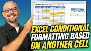
Excellent video! I learned that formatting based on cell B4 would involve highlighting the cells you want based on B4, and creating a custom conditional formatting rule with the syntax: =b4 followed by whatever. As an example, if you want any input into B4 to cause a change in font color, the sytax would look like this: =B4"" The is syntax for not equal, and "" is just double quotes around nothing. Good stuff :)
Gosh, you made this so easy! Thanks tons! And you have a great FM radio deejay voice too, so that helps. You're kinda the Bob Ross of Google Docs, right? 🤓
Nice video I have question please How can I make the other values in the same row appear .I have one cell in each row get it value from ifttt and nodemcu and I put condition that if the value equals to 1 for example in the same row 2 cells value will appear. Can you tell me how to do it please
Based on your sheet: I'm looking for a way to add together the total amount of units sold by Joan and displayed in a separate cell or graph. How would this be possible?
Very Helpful. Just what I wanted, thank you. Is there a formula for other cells in the row to change colour based on cell colour rather than value please? Thank you
What's missing here is how to define the actual format of the cells you have chosen using the conditional statement. My sheets only has a couple of formats and a line that says "Custom Format" but clicking on that has no effect. I can only choose from the predefined six options. I've Googled and can't find any way to create a new "custom format" (in my case I want to put a line between the rows when the value changes).
Conditional formatting is just for formatting existing data in existing cells. Adding a line is outside of the scope of what formatting does. I would guess that you could accomplish this using a script.
Came here looking for a refresher on what formula syntax to use to get conditional formatting based on cells above or below the current row. I know it's possible, because I did it before, but understandably not a common application. Thanks!
If it is a fixed number above or below, then just make the row number that amount higher or lower in the custom formula. However, I have a feeling that I'm missing the crux of your question but I'm not sure.
I have a spreadsheet that gets rows automatically added every day or so. In a column (D) with steadily increasing whole numbers (1,1,2,3,3,3,4,5,6,6,7,7,7 etc.), I wanted the very last (most recent) to be highlighted using conditional formatting, omitting duplicates. In other words, the first "7" of my sample list, not all three "7's". Here's how I got that to happen this morning, after posting my comment to you. I set up a rule that applies to "D7:D1007" (the range should automatically expand as rows beyond 1007 get added), and gave it a "Custom Formula" of =AND(D7=MAX(D:D),D7D6) This formula will only match (that is, become TRUE for and consequently highlight) a single cell in Column D, namely the number that is both bigger than all the others AND not equal to the value in the cell immediately above it. Thanks for heading me off in the right direction!
I appreciate your videos, they have helped me. I'm looking for a video that will show me how to automatically enter text, "yes or no" into a new column based on the value of column in that row.
I am learning a lot with your videos. Thanks a lot sir.... great job. You are the best teacher!!! I want to know if you have a video which explain if the hour that you have scheduled in a cell has passed using the hour of the computer. An example: you had to call somebody at 9:00 am and wrote it in a cell but now the time is 10:00 am. How to use the format to change the color of the cell if the time has gone by.
Love your videos, they have taught me so much! Is there any way to make the color from 'sheet 1' to then match the drop down selection of 'sheet 2'?? TIA!
Very instructive. Do you have a vid with a similar example but for when the cells in one sheet are being compared to cells on a different sheet? Perhaps using the Indirect function? I've been trying to use Indirect since I've noticed ppl around the web mentioning that it can be done using that one function, but I have yet to crack it. My equation in conditional formatting doesn't give me an error message but it just won't do what it is supposed to do in terms of the formatting. Any help much appreciated. Thanks. Great video btw.
I know I had a similar conversation to this, but I looked and can't find it now. I think it ended up at the INDIRECT solution as well. I am assuming you mean another sheet in the same file. If it's a different file, you could try IMPORTRANGE.
@@ProlificOaktree Yes, a diff sheet but same file (or workbook). It's actually a Google Sheets spreadsheet tho, not a desktop Excel file. Anyway, for range to be conditional formatted in Sheet 2, this is my cond formatting: Range formatted in Sheet 2: C6:P23 Formatting function: =COUNTIF(INDIRECT("Sheet 1!$C$6:$P$23"),C6)=0 Formatting: Just wanted to have all the cell contents in Sheet 2 (the table with the formatting) that are different from their corresponding matching cells in Sheet 1 appear in bold. Both sheets have similar tables in size and structure, so they are basically identical. But some of the values in Sheet 2 change over time. So I just want to have the values show in bold when/ if they change. Anyone can spot a mistake in there please give me a heads up. It's kind of weird though that when I do it with smaller sized data in another sheet, the conditional formatting works just fine. The values that have changed appear in bold as intended. But in the one sheet (with more rows & columns) that I want to actually format it doesn't work. If there's anyone that has used Google Sheets and has encountered this problem before pls let me know. Thnx
Maybe this sounds crazy, but I want for the formatting in a cell containing text to match the formatting in a cell containing numbers, but that cell containing numbers also has conditional formatting based on a color scale with other number cells. Any ideas on how to go about doing that?
Can you help ? I have created an expense income sheet. When an expense is made by credit care, I would like to the sum to subtract from the row which contains the running credit card balance as well as subtract from the row which contains the overall balance.
You could have a credit card only column and pull numbers into is using something like =IF(A1="Credit Card",B1). If A1 was the description field and B1 was the amount.
Very helpful. So basically: As the conditional formatting evaluation is moving through the range, cell by cell, each cell being evaluated is considered the new relative A1 (first column, first cell) to the formula with B2. Therefore: B2 indicates that the second column, second row (B,2) *relative* to the current cell being examined. A1 through G1, A2 through G2, all the way to A1000 to G1000 (upper max of 1,000 rows examined). However, we can break that *relative* processing. $B2 indicates that regardless of the current cell being examined (A1 through G1000), the formula should always only apply to the sheet's B2 cell, and NOT relative to the current cell being iterated. OP: Does that sound accurate?


Very helpful. Millions of videos on conditional formatting but yours was what I was looking for.
indeed
Those birds and nature sounds in the background was oddly soothing and perfect as background noise for something technical like this. Well done.
Thank you! Those are Pennsylvania birds...
I usually prefer written article over videos because most of the people just ramble endlessly before going to the point. But for this particular query, there is no match. There are tons of videos and articles that show you comparing cell values like 20 etc but nothing on = value. Most notably "string" value. Conditional formatting based on another cell's "string value"? There is none except this video. And the creator understands well how and when to slow down the mouse pointer so noobs like me can follow where you're going. Best tutorial in all category. Period.
Whew, thanks! I love that this video is still helping people after so long.
Thank you! I recently got a promotion to Operations Coordinator at my job, and we work in Google Sheets daily. I was nervous due to the video being 3 years old, but Google Sheets hasn't changed, and you've made my job much easier with your great tutorials. Thanks again!
Glad it was helpful!
@@ProlificOaktree Hi, how can I make it, so it colors whole row.
Excellent, within the first 2 min you taught me exactly what I needed. Bonus, I learned A1:A highlights the whole column. Thanks!
For what it's worth, I learned the A1:A technique for the first time as I was researching this video.
Close enough to what I was looking for, to point me in the right direction. Thanks!
The $ sign in the custom condition is EXACTLY what I was looking for. Thanks!
Glad I could help!
Spent an hour tinkering with the sheets help section and watching other videos. I quickly learned that watching anyone but you is a waste of time. Liked and subscribed, thank you for your work in helping educate users on how to use Sheets!
That's a great compliment, thanks! It's good to have you around.
I was looking for a training video for a colleague and I found this one. I've been using spreadsheets for more than 20 years. This is the most comprehensive and enjoyable video I've ever seen on the topic and I learned a few things!
That's a great compliment, thank you!
This wasn't *exactly* what I needed, but it definitely helped me make the logic jump to get to what I needed. Thank you!!
You're welcome!
I've seen lots of Google Sheets video but usually don't learn much because they are too fast for someone learning it. This I find is one of the clearest videos I've seen. You should develop and sell a Google Sheets online course if you don't already.
Oh, thank you. I have done that and develop was the easy part! Still working on the sell side of things.
When I couldn't figure it out by reading 3 pages of Google search, you did it in 3 minutes. Thanks!
Thanks, I'm glad it helped you out.
Problem solved and straight to the point video! Thank you!
Glad you liked it!
First person to explain the use of $ sign in a way I understood. Didn't even come here for that. Thank you.
Game changer
it's rare for me to find exactly what i was looking for in the first video, but this was it - awesome, thank you!
Wow, that's a great compliment! Thank you.
Really Cool Video. Five Years Later, and still helping!!
Thanks Alex. I still remember making this one. Glad you're still using it.
Many thanks!!! I've been spinning and spinning looking for a solution. Thanks again
This is EXACTLY what I was looking for! Thanks!!
Boom!
I tried figuring this out a month or two ago and gave up. Your video finally reveals how! Thank you thank you!
You're welcome! I'm glad it helped you out!
I've watched several of your tutorials and I'm not a teacher or a student. Excellent for any person using the program. Thanks for your time and keep up the good work!
Hey, thanks! I appreciate the thoughtful feedback.
This was the exact answer I was looking for! Thank you very much.
EXACTLY what I needed. Thank you, thank you And THANK YOU for just diving right in and solving the problem pronto. You had a clear video name and did that exact thing within the first few minutes.
You are a rockstar and your video just saved me from throwing in the towel.....you're a lifesaver!!! THANK YOU!
Thank you so much! This solved my issue perfectly!
This is a great video! I have worked for years with Sheets and I was unable to format cells based on other cells, and now it is a piece of cake. Thanks for sharing this great content! Cheers.
Glad it was helpful!
It's so easy when you know how. This has been a great help. Thanks.
Glad I could help out!
Extremely helpful, even in 2024! Thank you!
Glad it's still helpful!
Came here troubleshooting
The $ thing to stop the formula from moving a variable was my problem, didn't know about it. God sent video
Wish you an excellent day!
A six year old video which exactly solved my problem... plus the original video creator is still answering comments. You sir have won the internet today.
You're observation is so 🔥 bro.
After more than an hour with google, your video was the first page that gave the answer I needed. All others missed to specify that custom formula should be preceeded by = to function correctly. Fixed my problem immediately! Great work. Thank you #prolificoaktree
EXACTLY what I needed. Thanks dude. And THANK YOU for just diving right in and solving the problem pronto. You had a clear video name and did that exact thing within the first few minutes. THANK YOU! I hate it when I know the answer I need will take a few seconds and all the videos I find are 15 minutes long. So thanks again.
Thanks for taking the time to let me know that you liked it and why. I have played around with longer intros but I almost always delete them because they seem boring me when I go back to edit them.
Very well explained - great stuff. Not many videos are this easy to follow. And thanks for not blowing your own trumpet with pointless graphics.
Thanks, I'm glad you like it. You're making me question the short intro graphics that I have on my newer videos now!
@@ProlificOaktree yep. If you want people to engage with you don't stop them. No one likes the credits on tv shows and YouTibe ads annoy people.
Love the fact that you just grey straight to the point. Not many people understand online training like you do - we can pause and rewind if we don't understand something so there is no need to re-explain something.
Well done :)
I spent a fortune designing up a super cool intro (and outro) for my videos. I loved it - but no one else did.
Thanks for sharing! Exactly what I was looking for.
the perfect answer to the question. Thank You!
You are welcome!
Love the birds chirping in the background
Thank you for this to the point video!
:)
Wow - thank you!! SO helpful, thorough and timely.
Exactly what I was looking for, perfect video.
Can you do this for AND? That is set cell color either in the same column or another column based on two values within the cell. E.g. if the text in the cell is 5 Day Diet Guide Ebook, I need to highlight the cells containing BOTH the words "Diet" & "Ebook". Is that possible?
Yeah, you write it with a similar method but put an AND at the beginning and then write two functions. Try it in an empty cell in the spreadsheet first.
@@ProlificOaktree Thank you for your response. It didn't work, I mean the formula in the video. I tried that on the spreadsheet and it returned FALSE. I typed on a different cell =A5="order", which returned false but that word was in cell A5.
And the same for the formatting, nothing happens. What am I doing wrong?? :/
Thank you so much for this video, I thought this was only possible in Excel
I use this video EVERY time I need to do conditional formatting. Thank you so much for sharing.
I know what you mean. The whole thing with fixing the column reference is not an obvious solution.
wonderful explanation - cheers mate!
Seriously you are a life saver!!!
Ah, my issue was the $ missing from the referenced cell. I didn't realize it was moving down from the specified cell every time you drag the Conditional Formatting down a row. The app makes it seem like every cell is still referencing the same cell as listed in the first row! Thanks!
Absolutely brilliant piece of work. Thank you
Excellent video! I learned that formatting based on cell B4 would involve highlighting the cells you want based on B4, and creating a custom conditional formatting rule with the syntax: =b4 followed by whatever. As an example, if you want any input into B4 to cause a change in font color, the sytax would look like this: =B4"" The is syntax for not equal, and "" is just double quotes around nothing. Good stuff :)
Exactly what I needed explained. Thank you!
youre a wizard for guessing why i came to your video haha
wish I could give you more than 1 like. thank you
Incredibly well explained! Thank you!
This was extremely helpful. Awesome job walking through the steps.
Thanks for this video - I was struggling with the syntax to get the custom formula to run across the whole row. Nice video!
Wonderful video, shared with someone that may try it themselves. Learning is all about trying over and over, it till you get it or close enough.
Yeah, just start doing it.
Gosh, you made this so easy! Thanks tons! And you have a great FM radio deejay voice too, so that helps. You're kinda the Bob Ross of Google Docs, right? 🤓
Ha, I love that compliment! Bob Ross is wonderful.
Great video, saved me a ton of time reading support docs.
Cool, glad to hear it.
Thank you sir, very helpful in making my report better.
Thank you. Perfectly explained
Glad it was helpful!
This helped me. Thank you
Great tutorial! First time trying it! Thanks!
Sweet!
This was so helpful, clear and simple. Thank you
Thank you so much for taking the time to do this, you're a lifesaver!!!
Well, thanks. I'm glad it helped you out!
Perfect dude. I learned something new about using dollar signs with cell references
Cool. Fixing cells comes in handy a lot so you'll probably be using it often.
BINGO! Very easy and to the point videos. Keep it up! I love learning something new with excel!
Glad you liked it!
EXACTLY what I needed. Thank you!
You're welcome. I don't know how anyone would figure that out by themselves.
Nailed it. Simple and clear, thank you!
You're quite welcome!
Thank you very much! great feature that you show here
AMAZING video!! Hero!! Thank you so much!!
You're welcome!
Nice video
I have question please
How can I make the other values in the same row appear .I have one cell in each row get it value from ifttt and nodemcu and I put condition that if the value equals to 1 for example in the same row 2 cells value will appear.
Can you tell me how to do it please
I like your conditional formatting tutorial on google sheets. Thanks.
I'm glad you liked it, thanks.
thank you for this!! I got the gist within 2 minutes. Diolch!!
Based on your sheet: I'm looking for a way to add together the total amount of units sold by Joan and displayed in a separate cell or graph. How would this be possible?
Maybe something like =SUMIFS(E2:E44,B2:B44,"Joan")
Your videos are really helping sir!!! Thank you so much :)
Super helpful video! Thank you for providing thoughtful context and explanation of how to make the custom formulas work for your needs.
Thank you!! Exactly what I was looking for! Explanation was very clear.
Thanks for the kind feedback. It makes it more rewarding for me.
The dollar sign is magical!
Very Helpful. Just what I wanted, thank you. Is there a formula for other cells in the row to change colour based on cell colour rather than value please? Thank you
Not that I'm aware of.
Exactly what I needed! You're a wizard! Thank you!
You're welcome. I'm glad it helped you out.
this was extremely helpful, thank you
Glad it was helpful!
Exactly what I was looking for! Thank you!
What's missing here is how to define the actual format of the cells you have chosen using the conditional statement. My sheets only has a couple of formats and a line that says "Custom Format" but clicking on that has no effect. I can only choose from the predefined six options. I've Googled and can't find any way to create a new "custom format" (in my case I want to put a line between the rows when the value changes).
Conditional formatting is just for formatting existing data in existing cells. Adding a line is outside of the scope of what formatting does. I would guess that you could accomplish this using a script.
Came here looking for a refresher on what formula syntax to use to get conditional formatting based on cells above or below the current row. I know it's possible, because I did it before, but understandably not a common application. Thanks!
If it is a fixed number above or below, then just make the row number that amount higher or lower in the custom formula. However, I have a feeling that I'm missing the crux of your question but I'm not sure.
I have a spreadsheet that gets rows automatically added every day or so. In a column (D) with steadily increasing whole numbers (1,1,2,3,3,3,4,5,6,6,7,7,7 etc.), I wanted the very last (most recent) to be highlighted using conditional formatting, omitting duplicates. In other words, the first "7" of my sample list, not all three "7's".
Here's how I got that to happen this morning, after posting my comment to you. I set up a rule that applies to "D7:D1007" (the range should automatically expand as rows beyond 1007 get added), and gave it a "Custom Formula" of =AND(D7=MAX(D:D),D7D6)
This formula will only match (that is, become TRUE for and consequently highlight) a single cell in Column D, namely the number that is both bigger than all the others AND not equal to the value in the cell immediately above it. Thanks for heading me off in the right direction!
Exactly what I needed. Thanks!
Thank you
Thank you, helped me a lot to know how to compare to one cell in particular
I appreciate your videos, they have helped me. I'm looking for a video that will show me how to automatically enter text, "yes or no" into a new column based on the value of column in that row.
Really a life-saver! Great tutorial!
Excellent work, thanks
Thanks for a clear concise tutorial!
Hi, when creating charts how do you select data for the horizontal and vertical axis in google sheets for Android?
Really helpful, clear video. Thank you!
THANK SIRR, YOU HELP ME A LOTT!
That's great example! Thanks you very much!
You're welcome.
I am learning a lot with your videos. Thanks a lot sir.... great job. You are the best teacher!!! I want to know if you have a video which explain if the hour that you have scheduled in a cell has passed using the hour of the computer. An example: you had to call somebody at 9:00 am and wrote it in a cell but now the time is 10:00 am. How to use the format to change the color of the cell if the time has gone by.
Put this is the custom formula box in the conditional formatting menu =IF([cell_with_time]>NOW())
@@ProlificOaktree waaaaaaaaaaoooooo.... this is fantastic. Thank a lot sir. You are a master.!!!!! It is working now.
Love your videos, they have taught me so much! Is there any way to make the color from 'sheet 1' to then match the drop down selection of 'sheet 2'?? TIA!
Very instructive. Do you have a vid with a similar example but for when the cells in one sheet are being compared to cells on a different sheet? Perhaps using the Indirect function? I've been trying to use Indirect since I've noticed ppl around the web mentioning that it can be done using that one function, but I have yet to crack it. My equation in conditional formatting doesn't give me an error message but it just won't do what it is supposed to do in terms of the formatting. Any help much appreciated. Thanks.
Great video btw.
I know I had a similar conversation to this, but I looked and can't find it now. I think it ended up at the INDIRECT solution as well. I am assuming you mean another sheet in the same file. If it's a different file, you could try IMPORTRANGE.
@@ProlificOaktree Yes, a diff sheet but same file (or workbook). It's actually a Google Sheets spreadsheet tho, not a desktop Excel file.
Anyway, for range to be conditional formatted in Sheet 2, this is my cond formatting:
Range formatted in Sheet 2:
C6:P23
Formatting function:
=COUNTIF(INDIRECT("Sheet 1!$C$6:$P$23"),C6)=0
Formatting: Just wanted to have all the cell contents in Sheet 2 (the table with the formatting) that are different from their corresponding matching cells in Sheet 1 appear in bold. Both sheets have similar tables in size and structure, so they are basically identical. But some of the values in Sheet 2 change over time. So I just want to have the values show in bold when/ if they change.
Anyone can spot a mistake in there please give me a heads up. It's kind of weird though that when I do it with smaller sized data in another sheet, the conditional formatting works just fine. The values that have changed appear in bold as intended. But in the one sheet (with more rows & columns) that I want to actually format it doesn't work. If there's anyone that has used Google Sheets and has encountered this problem before pls let me know. Thnx
Thank you very much, this helped me a lot and is exactly what I'm looking for. Keep it up.
Glad it helped!
Maybe this sounds crazy, but I want for the formatting in a cell containing text to match the formatting in a cell containing numbers, but that cell containing numbers also has conditional formatting based on a color scale with other number cells.
Any ideas on how to go about doing that?
Can you help ? I have created an expense income sheet. When an expense is made by credit care, I would like to the sum to subtract from the row which contains the running credit card balance as well as subtract from the row which contains the overall balance.
You could have a credit card only column and pull numbers into is using something like =IF(A1="Credit Card",B1). If A1 was the description field and B1 was the amount.
Thanks, This was very Helpful and concise
Thanks for this. Very helpful.
You're welcome, I'm glad you liked it.
How do you set the condition to be the text of the adjacent cell *_starting with_* certain characters?
Very helpful. So basically:
As the conditional formatting evaluation is moving through the range, cell by cell, each cell being evaluated is considered the new relative A1 (first column, first cell) to the formula with B2.
Therefore:
B2 indicates that the second column, second row (B,2) *relative* to the current cell being examined. A1 through G1, A2 through G2, all the way to A1000 to G1000 (upper max of 1,000 rows examined).
However, we can break that *relative* processing.
$B2 indicates that regardless of the current cell being examined (A1 through G1000), the formula should always only apply to the sheet's B2 cell, and NOT relative to the current cell being iterated.
OP: Does that sound accurate?
Yeah, that sounds like the right concept to me.