Just worked through this series on Excel and accounts and found them very useful. Lots of things I learned from your clear explanations and I have much more confidence with pivot tables now. Many thanks.
This video was exactly what I was looking for, I thought it would be difficult to apply this, but it was so straight forward. Thank you for making this video.
Simon this is a great video, I've been watching and learning a lot of new skills thanks to you. I have a question which I have never seen explained anywhere ... are we able to highlight the Rows section in a pivot table based on the results from one or several of the columns in the Values section of the pivot? It would be similar to highlighting the Month on the row labels of your example on this video. Thank you for your help!!!
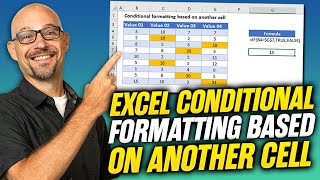
Great that my videos are of help to you Juan. 😁 Regarding your question I haven't found a way to add conditional formatting to the Rows in column A for month that will work as in the video for a Pivot Table. However, a workaround is using a conditional formatting formula such as =$B6>5000 then applying it to specific cells. The downside of this is that if you add more rows at the bottom they won't be included. It's not perfect by a long shot. But might work.
Great tutorial video. Have been looking for this answer for a while and finally here you bring it on a silver plate.. One question though, there is no way around to include the first row label? I get a message saying that I cannot apply CF to a range that has cells outside the Pivot Table data region.... Any comments please?
i don't see similar option, like you have for ex. "All Cells showing "sum of profit%" values this is something cannot see where can apply for all cells with the sum data
Good question those options only appear when you have the pivot table with those fields in selected. If you don't have the cells selected you won't see it. I selected cell E6 before I went to Pivot Table to make sure I could see All Cells showing "Sum of Profit%".
In the conditional formatting rules bix there should be an option so that you can make sure the rules applies are only on the Pivot Table. Conditional Formating - Manage Rules then use the drop down list at the top to apply the rules to the Pivot Table
@@computertutoring Thank you for you quick answer! Actually I found the mistake, instead of to drag the to Values, normally I only drag to rows, because this way I can filter by values as well, and when we drag to value, we don't have this option and we cannot apply conditional formatting according to the way that you explained. So to fix that, I just dragged from Rows to Values and now I'm able to do that. Thank you again.


Starter & Completed template file - www.computertutoring.co.uk/excel-tutorials/accounts-excel/pivot-table-conditional-formatting/
Just worked through this series on Excel and accounts and found them very useful. Lots of things I learned from your clear explanations and I have much more confidence with pivot tables now. Many thanks.
Thanks for the positive comment. I originally created these for friends who ran their own businesses glad it also helped you 👍🏽
You have no idea how much this has helped! Thank you for sharing!
Thanks Rock On Pivot Table Conditional Formatting 👊🏽
I have watched a lot of Excel videos. A great combination of how and why of doing things
Made my day thanks
Dear Simon , great video ... just helped me out of a problem in which i was stuck for almost an hour ... salute ..
Thanks! Love hearing comments like that.... so pleased it helped!😀
This video was exactly what I was looking for, I thought it would be difficult to apply this, but it was so straight forward.
Thank you for making this video.
That's what we love to hear!😀 Thanks
I like the flexibility to change the target and the formatting automatically updates! Cool.
Excellent video presentation.
Very useful tips and so well explained.
Thanks for sharing Simon.
Thanks for saying much appreciated
Thanks! It helped me with applying conditional formatting for all cells in the pivot table
👍🏽 Glad this Pivot Table tutorial helped
Simon I love your tutorials
Thanks for saying so 😊
Cool like the litte hack so you can format the whole, well nearly, row in the Pivot Table
Yeah not the fastest way but does the job
Thank you much!
And thanks again 😁
Thanks so much mate, very well explained 👍🏽
Glad it helped my friend
You Rock Simon! Cheers!
🎸🎸🎸
Thanks!
Thanks for saying
Fantastic 🔥
Thx 🙏🏽
you are best.
Awww! 😊
Thank you so much , i can do it , so great🥰👍👍👍
Simon this is a great video, I've been watching and learning a lot of new skills thanks to you. I have a question which I have never seen explained anywhere ... are we able to highlight the Rows section in a pivot table based on the results from one or several of the columns in the Values section of the pivot? It would be similar to highlighting the Month on the row labels of your example on this video. Thank you for your help!!!
Great that my videos are of help to you Juan. 😁 Regarding your question I haven't found a way to add conditional formatting to the Rows in column A for month that will work as in the video for a Pivot Table. However, a workaround is using a conditional formatting formula such as =$B6>5000 then applying it to specific cells. The downside of this is that if you add more rows at the bottom they won't be included. It's not perfect by a long shot. But might work.
Great tutorial video. Have been looking for this answer for a while and finally here you bring it on a silver plate.. One question though, there is no way around to include the first row label? I get a message saying that I cannot apply CF to a range that has cells outside the Pivot Table data region.... Any comments please?
Well actually I found it, I just applied created a new conditional format formula for the first column. Cheers
Adding another conditional formatting formula will do it cool
i don't see similar option, like you have for ex. "All Cells showing "sum of profit%" values this is something cannot see where can apply for all cells with the sum data
Good question those options only appear when you have the pivot table with those fields in selected. If you don't have the cells selected you won't see it. I selected cell E6 before I went to Pivot Table to make sure I could see All Cells showing "Sum of Profit%".
It does not clarify that any data refresh or filter change will wipe out any formatting. Also does not allow pivot table formatting based on text.
Good🥰
Cheers 😁
Thank you, that's been bugging me for years.
Glad it help mate 😉
Good video, but my excel doesn’t show that little square with thise 3 options
In the conditional formatting rules bix there should be an option so that you can make sure the rules applies are only on the Pivot Table.
Conditional Formating - Manage Rules then use the drop down list at the top to apply the rules to the Pivot Table
@@computertutoring Thank you for you quick answer! Actually I found the mistake, instead of to drag the to Values, normally I only drag to rows, because this way I can filter by values as well, and when we drag to value, we don't have this option and we cannot apply conditional formatting according to the way that you explained.
So to fix that, I just dragged from Rows to Values and now I'm able to do that.
Thank you again.
Can you color the 1st column based on formula !
Sorry haven't worked that one out inside a Pivot Table
Why too much work just to do conditional formatting for the entire row?
There is another way to hight whole row in one rule..
You can use a formula within conditional formatting however it can problematic with Pivot Tables.