Видео

That's just the percentage of the distribution below 0 and above 0. That annotation could have been omitted.

For a conceptual explanation of how to set priors, see this open-access article: Bayesian data analysis for newcomers, link.springer.com/article/10.3758/s13423-017-1272-1 In particular, see the section headed "Prior distribution: innocuous, hazardous, beneficial". For a detailed example of setting priors for a realistic yet simple application, see the Supplementary Example for this open access article: Bayesian analysis reporting guidelines, www.nature.com/articles/s41562-021-01177-7 The Supplementary Example is available here: osf.io/w7cph/

@@JohannZahneknirsche Thank you a lot, Prof Kruschke, The only reason that does not make me use the Bayesian approach is the possibility of having a bias in the analysis, the funny part is as I asked myself why the frequency approach does not have a bias as many researchers state, since sometimes the frequency models may not be the correct approach. I asked my professor if I can use the Bayesian approach in my research and he encouraged me to work only with the traditional approach he explained the traditional approach works very well in machine learning compared to Bayesian, but I am curious about how to choose the correct prior, especially for logistics and survival analysis. I want to read more about the bayesian approach and I may buy one of your books soon🙂 I encouraged you to make new videos prof, I found your explanation very clear and let us make this channel active again. Best regards, Amin

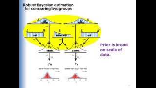
Dear Linford: Have you looked at the new data? Are the sample means closer together than they were before? (There should be no need to change the priors, because the scripts make the priors broad relative to the scale of the data.)

@@JohannZahneknirsche Hi John, thanks for your reply. The sample means are much further apart than they were (~90 units), which is why I was expecting [HDIlow,HDIhigh] for muDiff to not include 0.

Any advise on this John?

Yes.

The two approaches ask different questions. Bayesian asks about credibilities of parameter values given observed data, frequentist asks about error rates give hypothetical worlds. Neither question is necessarily the "correct" question to ask, but most people intuitively think they're asking the Bayesian question because they interpret the result in a Bayesian way.

Thanks for the reply, John. Yes, I agree that the two approaches ask different questions, and, as your examples nicely illustrate, can yield different conclusions to inform our decisions. Given the inherent flaws in NHST and the logical coherence of Bayesian inference, which one would you trust more to make decisions? I think I know the answer ;)

Sorry but the scripts assume you have no missing data. If your missing values are "missing completely at random" such that there is no systematic reason why some values are missing and not others, then simply delete the rows with missing values. Otherwise you have to model the missingness, which is a completely different ball game.

Felix, thanks for your interest. 1. The prior is explicit and must make sense to a skeptical audience. You can always show what happens when using different priors to satisfy the interest of skeptics; that's often called a "sensitivity analysis". Diffuse priors for parameter estimation have little impact on the posterior distribution. But priors for Bayes factors can be highly influential. In any case, strongly informed priors (using prior information everyone agrees on, such as in meta-analysis) can be very helpful to leverage small data sets. 2. For power analysis, when using a distribution of hypothetical values, the power estimate integrates across the uncertainty in the effect size. The difference is that small hypothetical effect sizes inflate the needed N more than large hypothetical effects sizes reduce the needed N. 3. The talk was not intended to contrast frequentist and Bayesian side by side to illustrate their differences. The talk merely tried to show some Bayesian approaches to the issues. For a comparison of frequentist and Bayesian, try this manuscript: ssrn.com/abstract=2606016

John K. Kruschke Thank you. That was very informative. Especially 2 is interesting to me.

Ops, looks like I skipped this part on the video. I also have the book but haven't reached this part yet!

Thanks for your interest. Hope the book serves you well!

+John Doe Actually it's natural log, for which log(3) = 1.1 approximately. The threshold for BF at 3 is just a conventional decision threshold like .05 for p values. Various proponents of BF's suggest different thresholds like 3 or 6 or 10, as applied considerations suggest. All of the details of the examples are in Chapter 13 of DBDA2E.

John K. Kruschke Thank you.

John K. Kruschke When doing random coin tosses I have noticed that sometimes there is a strong bias in the first ~20 trial, despite p=.5. The p value is of course low enough to reject the null, but the bayes factor also is extremely high and the HDI is clearly outside the ROPE. Clearly none of these can be used as a stopping rule.. right? Now one could also include the width of the HDI, but that means I'd need to do at least a few hundred coin tosses to make a conclusion... there's no free lunch I guess.

+John Doe Right, in small samples there is huge variability from one sample to the next. Because of this, some proponents of optional stopping require a minimal sample size before optional stopping is allowed. For example, you have to collect at least 20 data points, and only after that can you check for stopping.

John K. Kruschke Ok, then why do we use θ=0.5 for the null hypothesis, which is like using a betapdf(infinity, infinity) prior for H0? If we, for example, have done 20 flips then why don't we contrast H1 (uniform prior) with a H0 with a prior that is the average posterior of countless 20-flip fair coin experiments with the same uniform prior instead of taking the posterior of an endless run of fair coin flips (which results in the above infinity betapdf)? In my 20 flips example this averaged posterior, that will be used as prior for H0, can be approximated with a betapdf(5.69, 5.69). So using this as prior for H0 I get: The max log bayes factor for 20/20 or 0/20 heads changes from 10.8 to "just" 4.2. And for 15/20 it changes from 1.2 to a barely positive 0.01 At 10/20 it is less negative than with the original H0 .. of course! With just 20 trials there is large uncertainty even with a perfectly fair coin. Does that make sense to you?

only 5% of the time or less

Hierarchical models are a way of using all the players' data to simultaneously inform each individual player's estimate. The individual estimates get pulled toward the group mode(s). That "shrinkage" attenuates the extremeness of outliers. Assuming that at least some of those outliers were produced by randomly extreme data, the shrinkage has reduced false alarms. This is not to say that any particular hierarchical model is "correct". Merely that hierarchical models are a reasonably way to formally implement the prior knowledge that individuals fall into particular groups. For example, suppose you learn that a player named Varun got 1 hit in 3 at-bats. What is your estimate of Varun's probability of hitting the ball? Now suppose I tell you that Varun is a young kid at a neighborhood playground, or I tell you that Varun is a professional player. Your estimate changes, depending on your knowledge of what other players inform the estimate. Shrinkage pulls the estimate toward the mode of the other players in the group.

John K. Kruschke Thank you very much. That is the entire point of hierarchical models. I understood now. I will be very glad to see an online course in coursera on this topic from you.

Hey John, have you tried (r)STAN (mc-stan.org/) already? Should work pretty much as a drop-in replacement for rjags and should yield much better convergence.

Thomas Wiecki Yes, I'm trying it out. From your experience, have you found any hitches in using it? How about in learning to use it? Thanks.

John K. Kruschke So far it's been a pleasure and converting models from JAGS is simple enough. Also, the interaction between R and STAN is much better than rjags, which I find quite annoying at times (e.g. coda).

I much prefer the modelling language in STAN to that in BUGS / JAGS. Explicit data, parameter and model blocks, as well as variable declarations (e.g., floating point or integer, and setting limits) are great. The compiler seems to be a lot more informative as to errors; for example, if you've accidentally passed STAN a data value that's out of range of allowable values it will tell you so (because you coded it in your data declaration). Finally, in my experience models in STAN converge far faster (produce more effective samples in less iterations) than in JAGS. I heartily recommend STAN.

Is there a version of BEST for Matlab?

I'll check it out. I prefer to use Julia, and would like version of this.

the book got introduced to me as "the dogs" book :D