- Видео 15
- Просмотров 3 783
Pavol Bokes
Добавлен 22 апр 2012
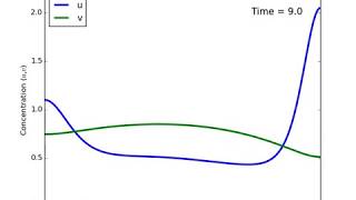
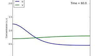
Turing instability - Dominant wavenumber k=8 - Example no. 7
The video shows the evolution of a solution (u,v) to a reaction-diffusion system
u_t = gamma*f(u,v) + u_xx, t > 0, 0 < x < pi,
v_t = gamma*g(u,v) + d*v_xx, t > 0, 0 < x < pi,
where pi=3.1415..., which is subject to Neumann boundary conditions
u_x = v_x = 0 at x=0 or x=pi,
and initial conditions
u(x,t=0) = u_0(x), v(x,t=0) = v_0(x), 0 < x < pi.
The reaction terms are given by the Schnakenberg reaction kinetics [1]:
f(u,v) = a - u + u^2 v
g(u,v) = b - u^2 v
All parameters (a,b,gamma,d) are provided inset.
The reaction-diffusion system has a unique spatially homogeneous steady state, which is stable with respect to spatially homogeneous perturbations.
However, Turing's instability occur...
Просмотров: 63
Видео
Turing instability - Dominant wavenumber k=8 - Example no. 6
Просмотров 347 лет назад
The video shows the evolution of a solution (u,v) to a reaction-diffusion system u_t = gamma*f(u,v) u_xx, t > 0, 0 < x < pi, v_t = gamma*g(u,v) d*v_xx, t > 0, 0 < x < pi, where pi=3.1415..., which is subject to Neumann boundary conditions u_x = v_x = 0 at x=0 or x=pi, and initial conditions u(x,t=0) = u_0(x), v(x,t=0) = v_0(x), 0 < x < pi. The reaction terms are given by the Sch...
Turing instability - Dominant wavenumber k=8 - Example no. 5
Просмотров 727 лет назад
The video shows the evolution of a solution (u,v) to a reaction-diffusion system u_t = gamma*f(u,v) u_xx, t > 0, 0 < x < pi, v_t = gamma*g(u,v) d*v_xx, t > 0, 0 < x < pi, where pi=3.1415..., which is subject to Neumann boundary conditions u_x = v_x = 0 at x=0 or x=pi, and initial conditions u(x,t=0) = u_0(x), v(x,t=0) = v_0(x), 0 < x < pi. The reaction terms are given by the Sch...
Turing instability - Dominant wavenumber k=3 - Example no. 4
Просмотров 367 лет назад
The video shows the evolution of a solution (u,v) to a reaction-diffusion system u_t = gamma*f(u,v) u_xx, t > 0, 0 < x < pi, v_t = gamma*g(u,v) d*v_xx, t > 0, 0 < x < pi, where pi=3.1415..., which is subject to Neumann boundary conditions u_x = v_x = 0 at x=0 or x=pi, and initial conditions u(x,t=0) = u_0(x), v(x,t=0) = v_0(x), 0 < x < pi. The reaction terms are given by the Sch...
Turing instability - Dominant wavenumber k=3 - Example no. 3
Просмотров 407 лет назад
The video shows the evolution of a solution (u,v) to a reaction-diffusion system u_t = gamma*f(u,v) u_xx, t > 0, 0 < x < pi, v_t = gamma*g(u,v) d*v_xx, t > 0, 0 < x < pi, where pi=3.1415..., which is subject to Neumann boundary conditions u_x = v_x = 0 at x=0 or x=pi, and initial conditions u(x,t=0) = u_0(x), v(x,t=0) = v_0(x), 0 < x < pi. The reaction terms are given by the Sch...
Turing instability - Dominant wavenumber k=1 - Example no. 2
Просмотров 277 лет назад
The video shows the evolution of a solution (u,v) to a reaction-diffusion system u_t = gamma*f(u,v) u_xx, t > 0, 0 < x < pi, v_t = gamma*g(u,v) d*v_xx, t > 0, 0 < x < pi, where pi=3.1415..., which is subject to Neumann boundary conditions u_x = v_x = 0 at x=0 or x=pi, and initial conditions u(x,t=0) = u_0(x), v(x,t=0) = v_0(x), 0 < x < pi. The reaction terms are given by the Sch...
Turing instability - Dominant wavenumber k=1 - Example no. 1
Просмотров 467 лет назад
The video shows the evolution of a solution (u,v) to a reaction-diffusion system u_t = gamma*f(u,v) u_xx, t > 0, 0 < x < pi, v_t = gamma*g(u,v) d*v_xx, t > 0, 0 < x < pi, where pi=3.1415... which is subject to Neumann boundary conditions u_x = v_x = 0 at x=0 or x=pi, and initial conditions u(x,t=0) = u_0(x), v(x,t=0) = v_0(x), 0 < x < pi. The reaction terms are given by the Schn...
Rosenzweig MacArthur 4
Просмотров 2678 лет назад
The video shows the dynamics of prey (x) and predator (y) populations which evolve according to the Rosenzweig MacArthur model [1] defined by x' = x(1-x) - axy/(a x), y' = -y/2 xy/(a x). Here we take a = 0.25. In the long term, the populations wind up onto a stable limit circle. The video was created for the purposes of teaching differential equations to students of mathematical finance at Come...
Rosenzweig MacArthur 3
Просмотров 2048 лет назад
The video shows the dynamics of prey (x) and predator (y) populations which evolve according to the Rosenzweig MacArthur model [1] defined by x' = x(1-x) - axy/(a x), y' = -y/2 xy/(a x). Here we take a = 0.5. In the long term, the populations converge towards a stable spiral. The video was created for the purposes of teaching differential equations to students of mathematical finance at Comeniu...
Rosenzweig MacArthur 2
Просмотров 2538 лет назад
The video shows the dynamics of prey (x) and predator (y) populations which evolve according to the Rosenzweig MacArthur model [1] defined by x' = x(1-x) - axy/(a x), y' = -y/2 xy/(a x). Here we take a = 0.8. In the long term, the population converge to a stable node. The video was created for the purposes of teaching differential equations to students of mathematical finance at Comenius Univer...
Rosenzweig MacArthur 1
Просмотров 9688 лет назад
The video shows the dynamics of prey (x) and predator (y) populations which evolve according to the Rosenzweig MacArthur model [1] defined by x' = x(1-x) - axy/(a x), y' = -y/2 xy/(a x). Here we take a = 1.5. In the long term, predators become extinct. The video was created for the purposes of teaching differential equations to students of mathematical finance at Comenius University in Bratisla...
Lotka-Volterra predator-prey model
Просмотров 9428 лет назад
The video shows the dynamics of prey (x) and predator (y) populations which evolve according to the Lotka-Volterra model [1] defined by x' = x(1-y) y' = y(-1 x) Each trajectory is a level set of H(x,y) = ln(x) - x ln(y) - y. The video was created for the purposes of teaching differential equations to students of mathematical finance at Comenius University in Bratislava, Slovakia. [1] Britton, N...
Schnakenberg's model
Просмотров 1368 лет назад
x' = a - x x^2 y y' = b - x^2 y a = 1/(6sqrt(3)) b =2/(3sqrt(3))
The chaotic attractor of the Lorenz system
Просмотров 1558 лет назад
The video shows the movement of three point particles in 3D space which are initially positioned at (x,y,z) = (i) (0,1,1.05) or (ii) (0,1,1.02) or (iii) (0,1,1,035); afterwards they evolve according to the Lorenz system of differential equations x' = s(y-x), y' = x(r-z) - y, z' = xy - b z, operating in the chaotic regime (s=10, b = 8/3, r=28). Starting close to one another, the particles remain...
Age-structured population dynamics
Просмотров 5408 лет назад
This educational video illustrates the dynamics of an age-structured population. The dynamics are obtained from iterations of a Leslie matrix [1], whose coefficients are adapted from [2]; the fecundities are increased for illustrative purposes. Ten thousand 15yo individuals (e.g. sea turtles in [2]) are initially present in the example. The video was created to complement a course on difference...


